
The prediction of electricity demand is vital for decision-making processes in the electricity sector. Decision making in this sector involves planning under uncertainty. One of the examples of this issue is to find the optimal day to day operation of a power plant and even strategic planning for capacity expansion. Therefore, the demand for electricity considered as the basis for power system planning, power security, and supply reliability. It is important to make very accurate forecasts to avoid the expensive consequences of underestimation or overestimation.
Electricity demand has unique characteristics; such it is non-storable, seasonal, and diurnal variations. Forecasting of electricity demand is essential for both electricity สล็อต system planners and operators; the only difference in their requirements is the forecast horizon. In the case of planners, the focus is on long term horizon, while for system operators, the focus is on medium to short term forecasts. Electricity demand based on the forecasting horizon can be divided into three categories: long term, medium-term, and short term. Long term forecast is used for taking policy decisions, system planning, and resource allocation. A medium-term forecast helps in planning yearly maintenance activities of power plants and monthly peak and energy demand management. In contrast, short term forecast helps in day to day operation of power plants and electrical network to manage daily loads effectively.
ANALYSIS
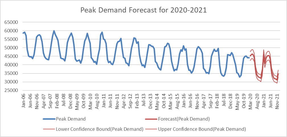
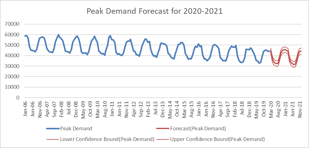
In this report, electricity demand in United Kingdom from 1st January 2005 to 29th February 2020 has been collected from National Grid that records the national demand every 30 minutes of the day. After that, the highest demand per month considered as the monthly peak demand for that month. The aim of this study is to find the monthly peak demand for the next year. Therefore, these peak demands for each month starting from January 2006 to February 2020 utilized to make a forecast for the rest months of 2020 as well as 2021.
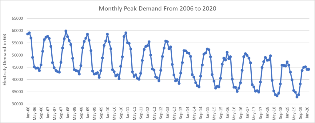
Figure (1) shows the monthly peak demand from January 2006 to February 2020. It can be seen from the pattern that there is a negative trend, and seasonal pattern every 12 months. Therefore, Holt-Winters’ seasonal method and Seasonal ARIMA used as forecasting methods, since it captures the seasonality, in addition to the trend.
- Holt-Winter Smoothing
This method involves a forecast equation and three smoothing equations, one for the level ℓt, one for the trend bt and one for the seasonal component st, with corresponding smoothing parameters α, and γ.
There are two types of variations: additive and multiplicative. Additive preferred when the seasonal variation is constant through the series, while multiplicative preferred when seasonal variations are changing proportionally to the level of the series.
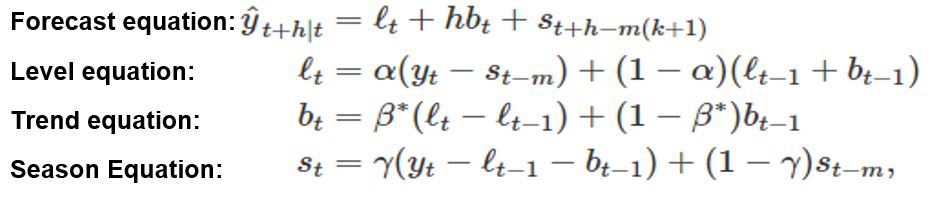
Figure (2) shows the decomposition of level, trend, and season, and it is clear that seasonal variation remains constant throughout the series. Therefore, additive variation has been used.
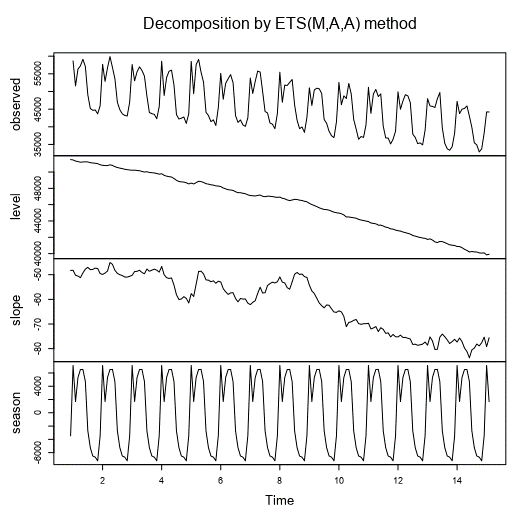
The smoothing parameters for this model are α=0.057504,= 0.001312 and γ= 1e-04. The model is shown in Figure (3).
This model shows the next error measures. It can be noticed that MASE is 0.6632, and MAPE is 2.08%, which means that this model achieves an accuracy of approximately 98% to predict the past monthly peak demand, which is quite good.
| ME | RMSE | MAE | MPE | MAPE | MASE |
| -122.5068051 | 1279.0187426 | 963.4039672 | -0.3292784 | 2.0821628 | 0.632336 |
2. Seasonal ARIMA
The seasonal ARIMA model incorporates both non-seasonal and seasonal factors in a multiplicative model. One shorthand notation for the model is ARIMA (p,d,q)×(P,D,Q)S. With p = non-seasonal AR order, d = non-seasonal differencing, q = non-seasonal MA order, P = seasonal AR order, D = seasonal differencing, Q = seasonal MA order, and S = time span of repeating seasonal pattern. Without differencing operations, the model could be written more formally as:
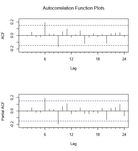
Figure (4) shows the Autocorrelation Function Plots that used to estimate the parameters of the model. Based on that, the models is ARIMA(1,0,0)(1,1,1)[12]. Figure (5) shows the model.
This model shows the next error measures. It can be noticed that MASE is 0.604, and MAPE is 2.00%, which means that this model achieves an accuracy of approximately 98% to predict the past monthly peak demand, which is better than Holt’s Winter in all error measures.
| ME RMSE MAE MPE MAPE MASE |
| 41.5008 1231.0978 925.2661 0.03468 2.0019 0.60415 |
CONCLUSION
In summary, making an accurate forecast will help the energy both providers and consumers to satisfy the demand and reducing the cost as well as to avoid the costly consequences of overestimation or underestimation. Electricity demand forecasting has three horizons: short, medium, and long in this report. A medium horizon forecast has been made for the monthly peak demand in United Kingdom to help in managing the electricity. Therefore, Holt-Winters’ and Seasonal ARIMA have been utilized, since it captures both the seasonality and trend. Both models show good performance in predicting the monthly peak demand with. But, Seasonal ARIMA shows better accuracy, since it has lower values in all error measures. As a result, forecasts have been made for the next 22 months using S-ARIMA. Also, it is recommended to update the data monthly in order to have more accurate and reliable forecasts.